Draw the Carnot cycle on the Temperature-Entropy plane. This will just be a rectangle on the T-S plane. The isothermal expansion and compression corresponds to horizontal segments because temperature is constant, while the adiabatic compression/expansion correspond to vertical segments, because zero heat exchange + quasistatic means entropy change is zero.
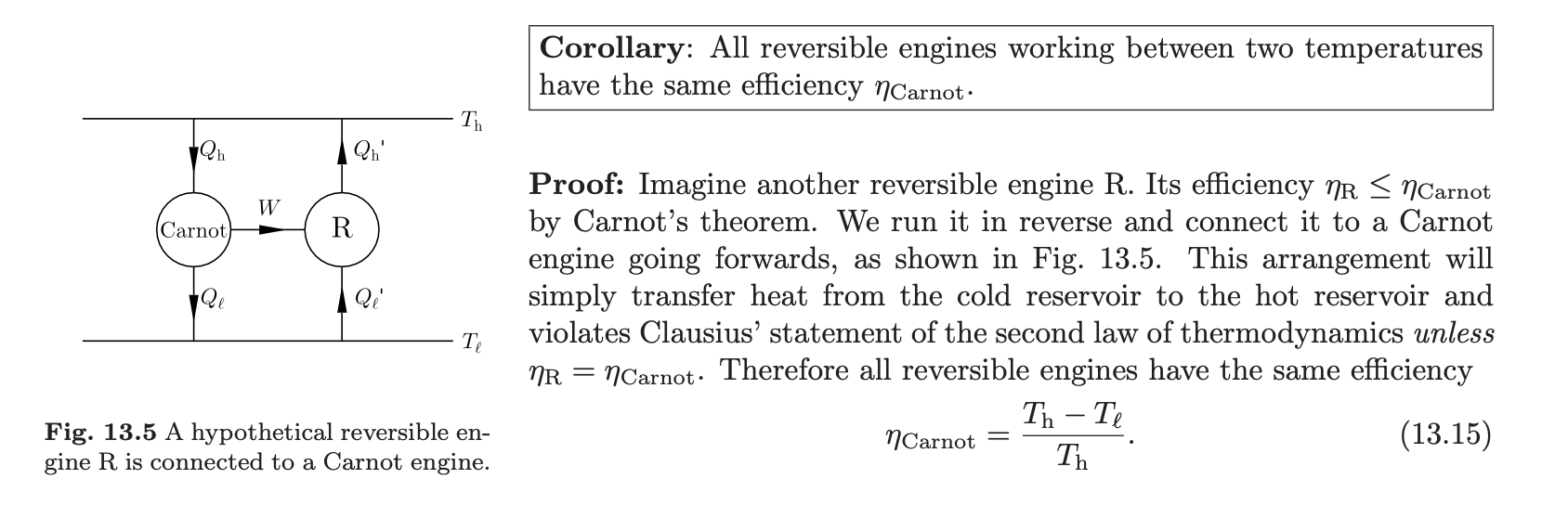
All reversible cycles operating between the same temperature difference have the same efficiency, which is the Carnot efficiency. However, implicit in this statement is that the reservoirs are designed in such a way that heat is always transferred at constant temperature.
Heat transferred between unequal temperatures is irreversible - generates entropy in the universe.
A quasistatic process can be represented on a PV diagram, and it has some efficiency one can compute. If we state that a process is also reversible, then it tells us something about how heat is drawn from the reservoir. In that case, we KNOW the efficiency is Carnot.
We observed for the Carnot cycle that the heat flowing into the system satisfies \frac{Q_{h}}{T_{h}} = \frac{Q_{l}}{T_{l}} Another way to say this is labeling the heat according to the segment, \frac{Q_{1}}{T_{1}} + \frac{Q_{2}}{T_{2}} = 0 The fluid returns to its initial state, so its change in entropy is zero. However, the reservoir will receive entropy
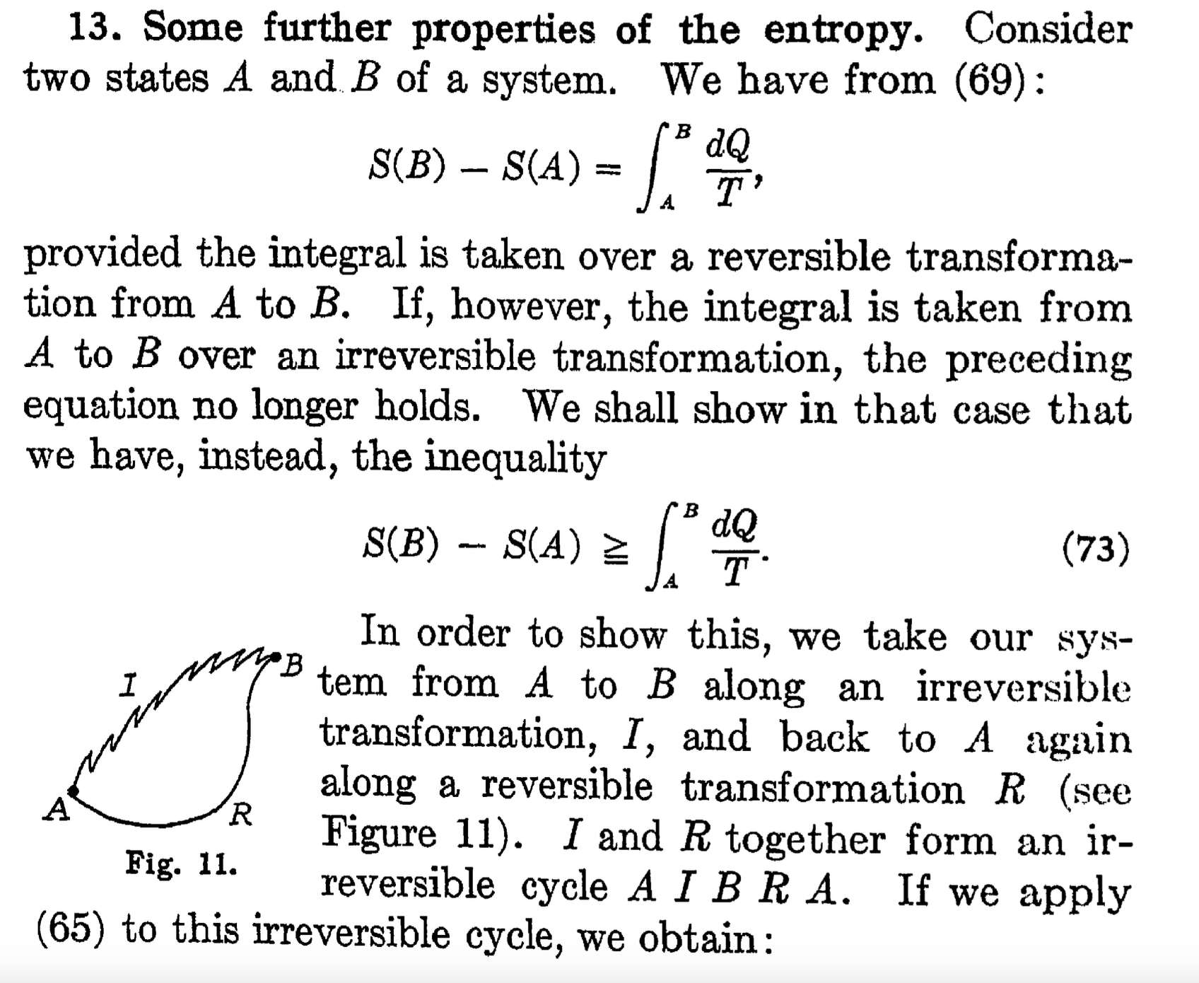
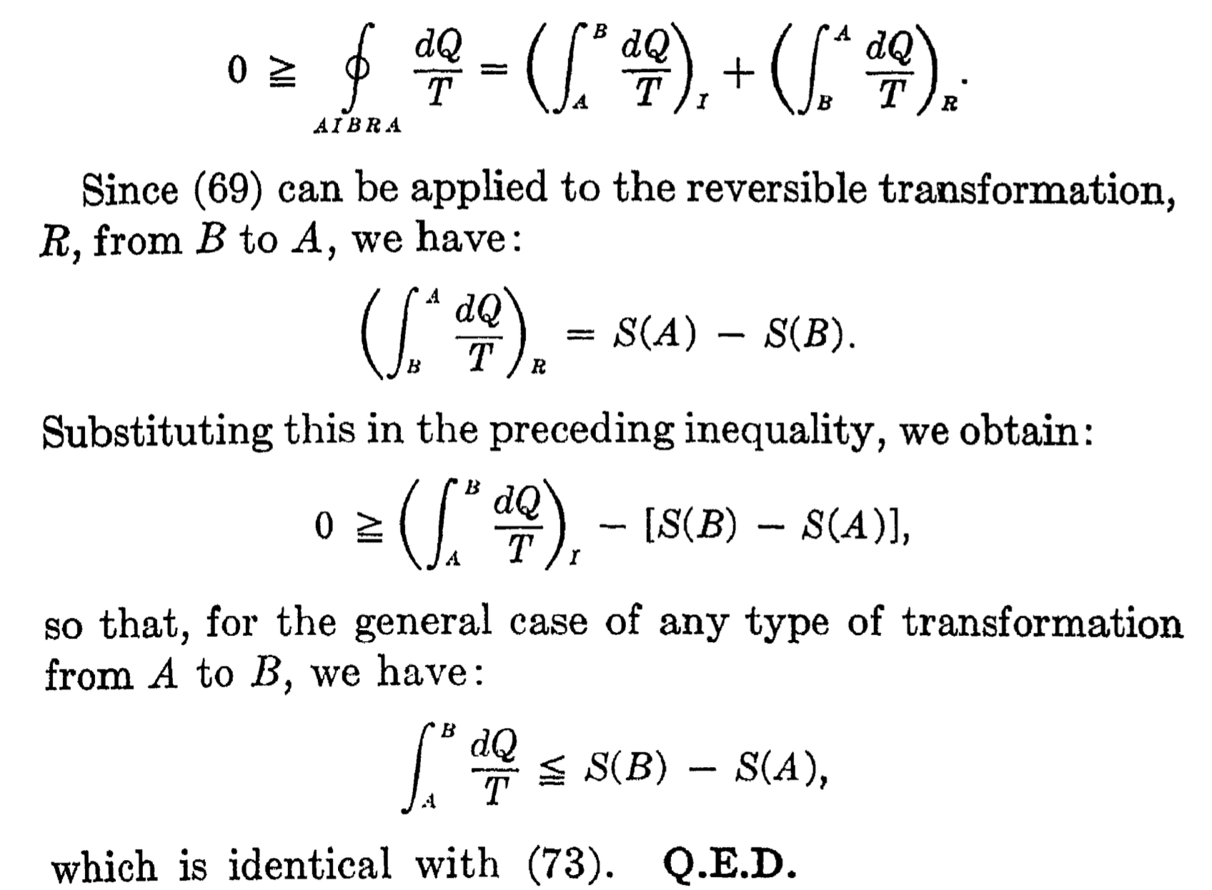
\Delta S_{res} =- \frac{Q_{1}}{T_{1}} - \frac{Q_{2}}{T_{2}} \ge 0 For more complicated processes, we can think about it on the T-S plane as an approximation of multiple carnot-like paths. In this case, we will have \sum_{i} \frac{Q_{i}}{T_{i}} \le 0 Or the continuous version \oint \frac{\bar{d}Q}{T} \le 0 Equality holds only for reversible processes. This is the Clausius inequality, which is equivalent to the second law of thermodynamics. Consider the following passage from Fermi’s Thermodynamics:
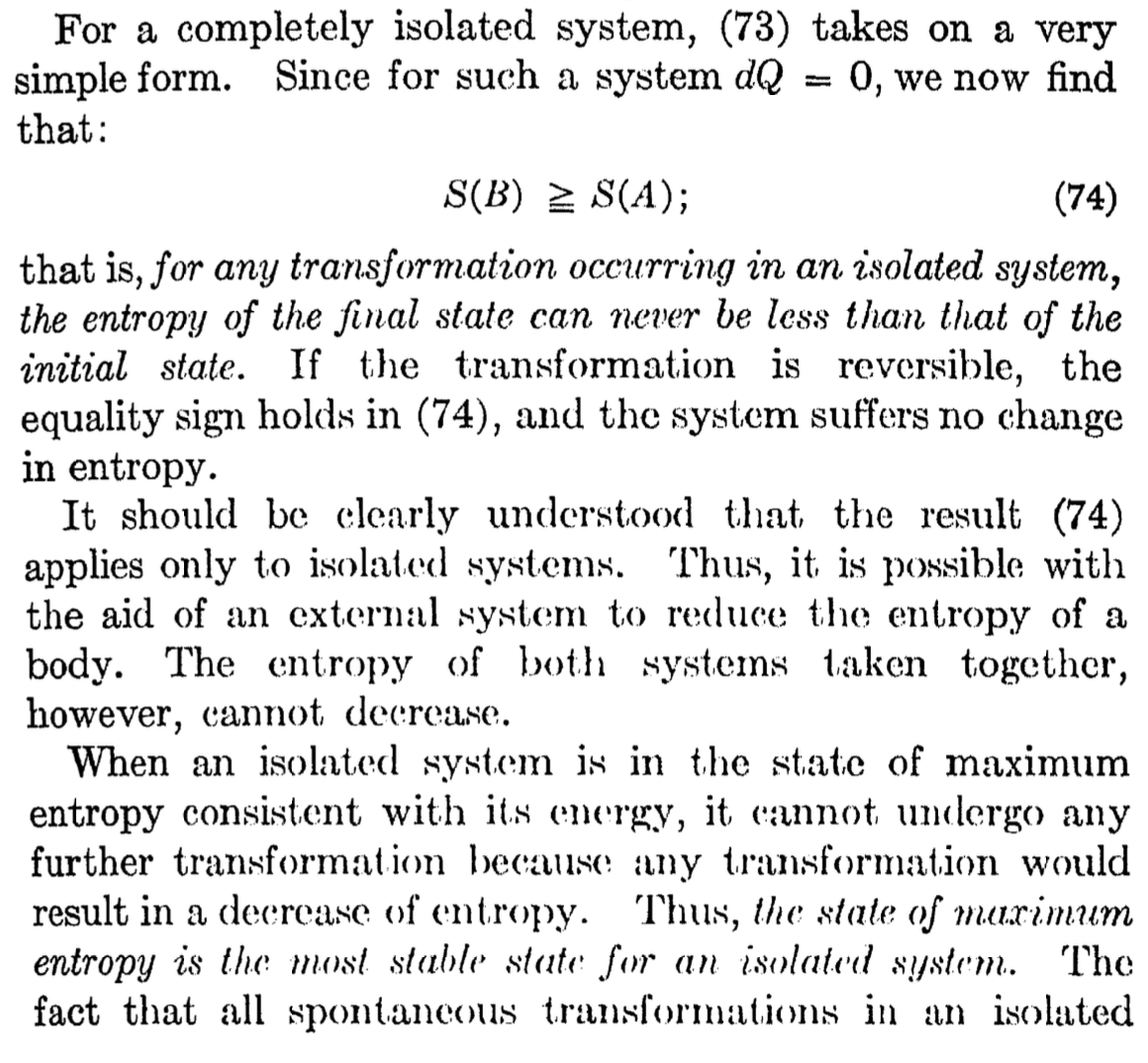
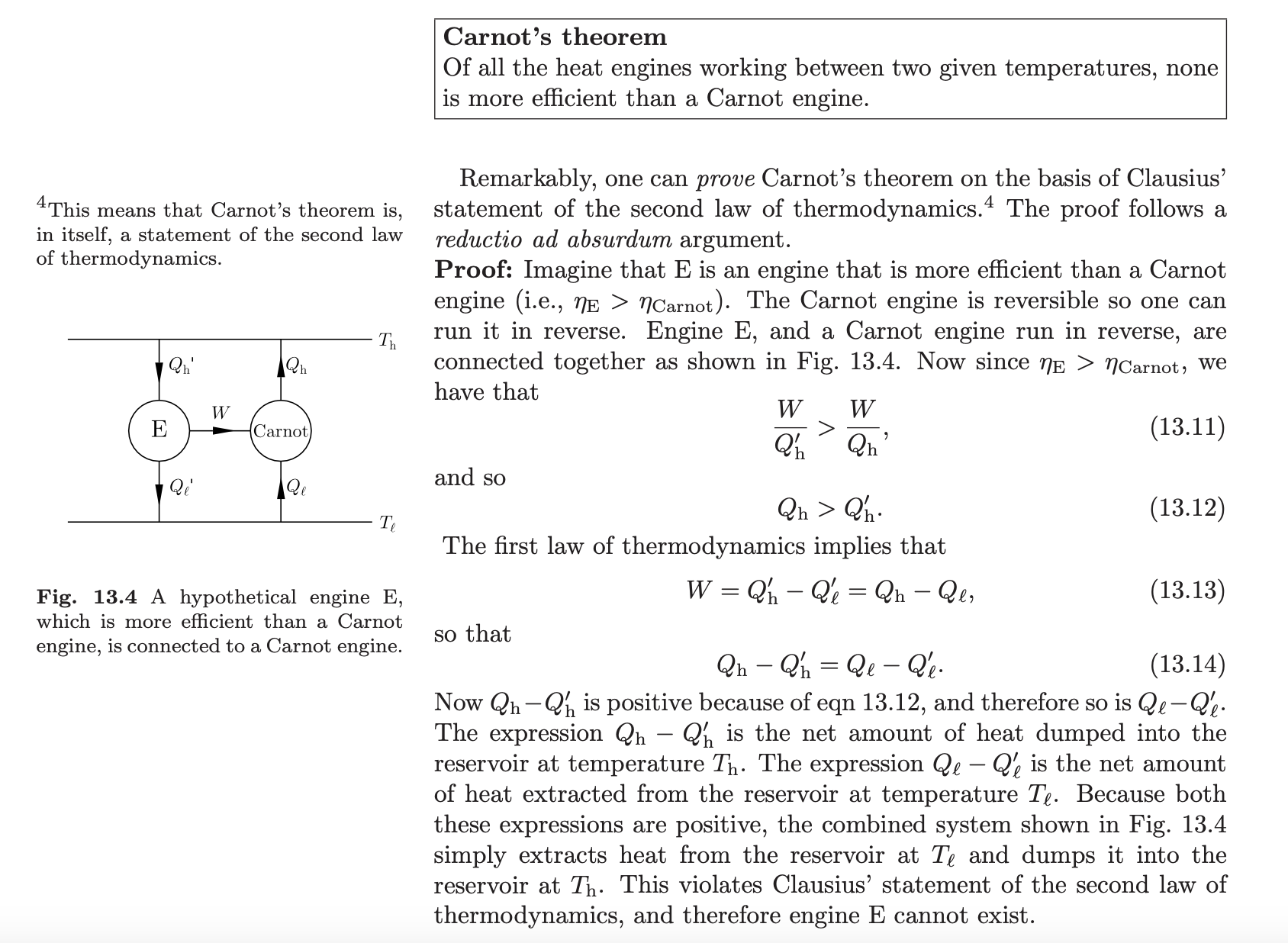
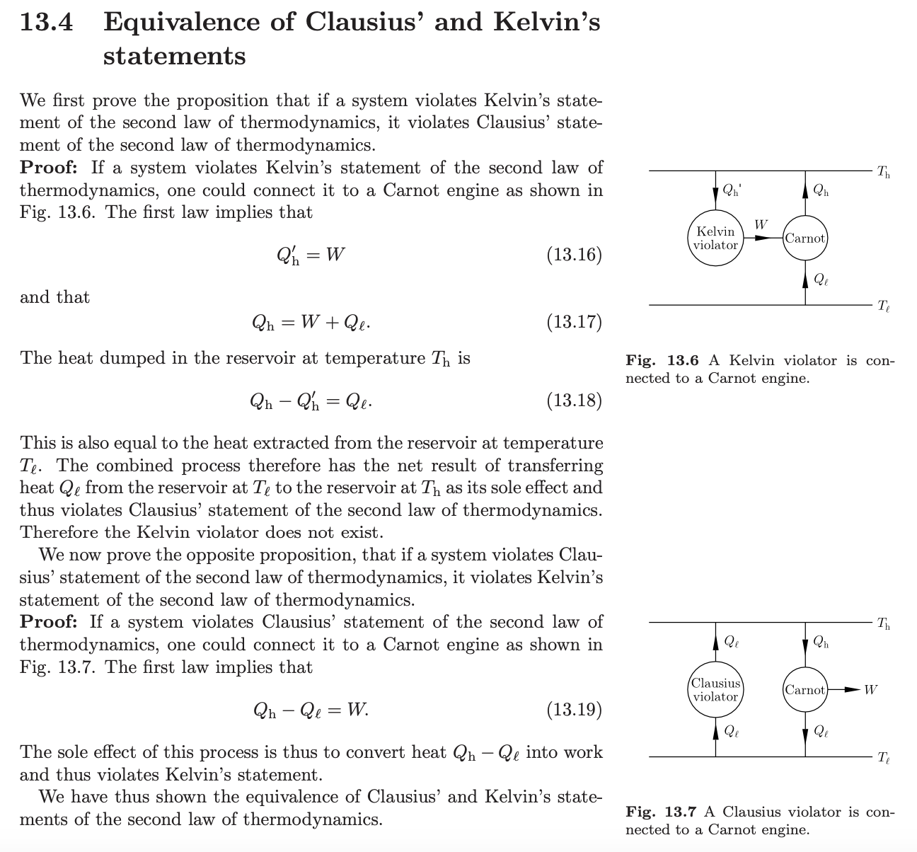
A note about the proof below. The Carnot engine efficiency is taken to be \eta_{C} = \frac{W^{by \, system}}{Q_{h}} = 1 - \frac{T_{l}}{T_{h}} When the Carnot cycle is reversed, the work done by the system now becomes work done on the system. However, the ratio stays the same. For the reversed Carnot cycle in Fig. 13.4 of the excerpt below: \frac{W^{on\, system}}{Q_{h}} = \eta_{C} = 1 - \frac{T_{l}}{T_{h}} However, the reversed Carnot cycle is now acting as a refrigerator, which means the metric of performance is no longer the efficiency but the so-called coefficient of performance: \epsilon = \frac{Q_{l}}{W^{on \, system}} Just as the Carnot cycle gives the optimal efficiency for a heat engine, it will give the maximal coefficient of performance. Having fixed the identity above, we know that W^{on \, system}+ Q_{l} = Q_{h} This implies \epsilon_{C} = \frac{Q_{l}}{Q_{h} - Q_{l}} = \frac{Q_{l}}{Q_{h}} \left(1 - \frac{Q_{l}}{Q_{h}}\right)^{-1} But note that \eta_{C} = 1 - Q_{l}/Q_{h}, which means we can write \epsilon_{C} = (1 - \eta_{C})/\eta_{C} = \eta_{C}^{-1} - 1 From the textbook Blundell & Blundell, Ch. 13: