In Chapter 2, Schroeder talks about systems with a constant energy. From the entropy and the energy, you then calculate temperature. That was the logic before. The temperature emerges as a description of a system at some fixed energy. You don’t need to know this, but this setting is typically referred to as the microcanonical ensemble. It just means you are considering a system of many particles that is at some fixed energy. We furthermore determined that at fixed energy, the fundamental postulate of statistical mechanics says that all accessible microstates are equally likely, so that the probability is uniform
P(s) = \frac{1}{\Omega(U)}
It is often more practical to speak about a system in contact with a huge reservoir at fixed temperature and a high heat capacity. High heat capacity means that the temperature of the reservoir is not affected by the system of interest. Therefore, the relevant setting here is not constant energy but constant temperature.
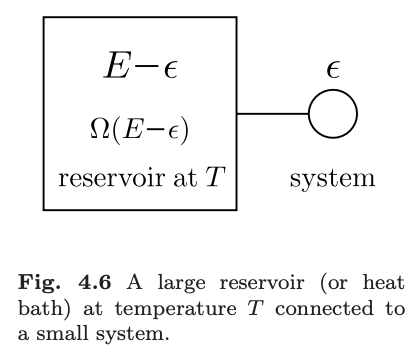
Start with a system in contact with a gigantic reservoir:
From Blundell and Blundell, Ch. 4
We fix the total energy to be E, and the temperature of the reservoir to be T. This will induce a distribution over the states of the system. The
P(\epsilon) \propto \Omega(E - \epsilon)
Expanding this for small \epsilon:
\ln \Omega(E - \epsilon) = \ln \Omega(E) - \frac{1}{k}\partial_{E} S(E) \epsilon
And using \partial_{E} S = \frac{1}{T} implies
\Omega(E - \epsilon) = \Omega(E) e^{ - \epsilon / kT}
From this we learn that the probability for the subsystem to be in the state with energy \epsilon is
P(\epsilon) \sim e^{ - \epsilon/ k T}
To get an actual probability requires normalization. The normalized probability for a configuration s is given by
P(s) = \frac{1}{Z}e^{ - E(s)/k T}
where the normalization factor in the denominator is called the partition function: Z = \sum_{s} e^{ - E(s)/kT}
Here the sum is over all possible microscopic configurations. In other words, over all the microstates.
What we can compute with a probability distribution like P(s) is the average value of certain quantities. Most relevant for thermodynamics is the average energy. This is given by
U = \langle E \rangle = \sum_{s} E(s) P(s) = \frac{1}{Z}\sum_{s} e^{ - E(s)/kT}
Notice a very cool identity. If I differentiate the partition function wrt T, I get
\frac{\partial Z}{\partial T} = \sum_{s} \frac{1}{k T^{2}} E(s) e^{ - E(s)/kT} = \frac{1}{k T^{2}} \sum_{s} E(s) e^{ - E(s)/kT}
Notice that this is very close to the average energy. In fact, I can get it into the right form by multiplying both sides by k T^{2}, and dividing both sides by Z:
k T^{2} \frac{1}{Z} \frac{\partial Z}{\partial T} = \langle E\rangle = U
The final trick is to notice that \frac{1}{Z} \partial_{T} Z is the logarithmic derivative, i.e.
\frac{1}{Z} \frac{\partial Z}{\partial T} = \frac{\partial}{\partial T} \ln Z
Putting it all together, we get an important identity for the partition function:
U = k T^{2} \frac{\partial}{\partial T} \ln Z
Recall in Lecture 13 that it is possible to get the internal energy from the Helmholtz Free Energy by taking derivatives. In particular, we saw that
-T^{2} \frac{\partial}{\partial T} \left( \frac{F}{T}\right) = U
Compare this to what we found above:
k T^{2} \frac{\partial}{\partial T} \ln Z = U
Inspires us to define:
F = -k T \ln Z
This is a very important and valuable relationship!
If we are thinking about a weakly interacting system, the energies are usually just the sum of the energies of the parts: E(s) = \sum_{i = 1}^{N} E_{i}(s_{i}). This implies that the partition function for N particles Z_{N}, can be written
Z_{N} = \sum_{s_{1}, ..., s_{N}} e^{ - \beta \sum_{i} E_{i}(s_{i})} = \prod_{i = 1}^{N} \left( \sum_{s_{i}} e^{ - \beta E_{i}(s_{i})}\right) = Z_{1}^{N}
where we have defined the single-particle partition function Z_{1} as the object in parenthesis, assuming
each particle has the same configurations and energies. To reiterate,
you can use this under two conditions: - Each particle has the same set
of energies, e.g. for the three-state system, E_{i} \in \{ - E, 0, +E\}, which is the same
for all N particles.
- The total energy is the sum of all individual energies for each
particle, i.e. E = \sum_{i = 1}^{N}
E_{i}.
Another interpretation of the Boltzmann probability comes from maximizing entropy.
There is a general formula for the entropy suggested by Gibbs:
S = -k \sum_{s} P(s) \ln P(s)
here P(s) is the probability of observing the system in a configuration s.
Exercise: What is the formula for the entropy if all microstates are equally probable?
When this is the case, the probability is independent of the particular configuration, and is just given by P(s) = \frac{1}{\Omega}, where \Omega is the total number of microstates. Plugging this in:
S = - k \sum_{s} \frac{1}{\Omega} \ln \frac{1}{\Omega} = k \ln \Omega
which is the familiar Boltzmann formula for entropy.
Next, I will introduce one of the most interesting and powerful concepts in statistical physics. It is one of entropy maximization. The Boltzmann distribution happens to be the distribution which produces the maximum entropy subject to a constraint on the total average energy.
Let’s define a function which we want to minimize:
L = -S + \lambda \left( \langle E \rangle - U \right) = k\sum_{s} P_{s} \ln P_{s} + \lambda \sum_{i} P_{s} E_{s} - \lambda U
( N.B. I have chosen to put s as a subscript instead of an argument in the P and E. This is just to avoid notational clutter, nothing more).
This function L(P_{s}) depends on all \Omega components of the probability P_{s} (there is one probability for each microstate, so \Omega probabilities total). We want to minimize this function subject to this constraint. This will end up maximizing the entropy subject to the constraint that the average energy, which is the one observable thermodynamic quantity we have access to, is constrained to be U.
Minimization of L is achieved by taking a derivative and setting it to zero:
\frac{\partial L}{\partial P_{s}} = k \left( \ln P_{s} + 1\right) + \lambda E_{s} = 0 Which implies
\ln P_{s} = -\frac{\lambda}{k} E_{s} - k, \quad P_{s} \sim e^{ - \frac{\lambda}{k} E_{s}}
We also must have this normalized, so
P_{s} = \frac{e^{ - \frac{\lambda}{k} E_{s}}}{Z}, \quad Z = \sum_{s} e^{ - \lambda E_{s}/k} In order to fix the constraint, we compute the entropy, take a derivative, and relate \lambda to the temperature.
Entropy is
S = - k \sum_{s} P_{s} \ln P_{s} = - k \sum_{s} P_{s} \left( -\frac{\lambda}{k} E_{s} - \ln Z\right) = \lambda U + k \ln Z
Differentiating wrt U
\frac{1}{T} = \frac{\partial S}{\partial U} = \lambda + U \frac{\partial \lambda}{\partial U} + k \frac{\partial \ln Z}{\partial U}
Next, we apply the chain rule to compute \frac{\partial \ln Z}{\partial U} = \frac{\partial \ln Z}{\partial \lambda} \frac{\partial \lambda}{\partial U} = - \frac{1}{k} U \frac{\partial \lambda}{\partial U} Inserting this into the equation above then gives
\frac{1}{T} = \lambda + U \frac{\partial \lambda}{\partial U} + k \left( - \frac{1}{k} U \frac{\partial \lambda}{\partial U}\right) = \lambda
We have thus related what is called the lagrange multiplier \lambda to the inverse of the temperature. Inserting this into the expression for P_{s} then recovers the Boltzmann factor.