 The derivative of the energy is the heat capacity. Below, we see how the
quantum heat capacity behaves vs. the classical heat capacity. Plotted
below is C_{V}/ k.
Beginning with a demonstration. I would like to reiterate what we are doing in this class. I will try to do it with a suggestive example. Which I will set up. Here is a collection of particles, moving in 1D. The left is a system of interest, the right is a large reservoir whose temperature we have fixed. Now we let the system relax. Notice that the microscopic dynamics is very simple. A particle moves at constant momentum, and reflects at a momentum influenced by the piston. Now, the particles in both regions are interacting, but only through the jiggling piston. How should we think about this system? There are too many particles to meaningfully follow all of the trajectories. It’s not interesting, and it’s not useful.
What does statistical mechanics tell us to do? It tells us that we should think about the system probabilistically. What does this mean practically? Imagine making a sequence of measurements of the velocities of this gas. After each measurement, we store the average measured value. After making many measurements, we plot the histogram. The resulting histogram, as we make more measurements, will approach the maxwell-boltzmann distribution. In other words, each measurement looks like a random variable sampled from a Boltzmann distribution. If this is true, then averages will approach expectation values measurements from this distribution. And all of the physics that we can possibly want can be obtained directly from this distribution. At this point, we decide to discard the dynamics completely, and just model our system probabilistically.
The classical harmonic oscillator is a very simple, but very useful example to study and understand many phenomena in physics. It is in essence just a particle of mass m attached to a spring with spring constant K. The equation of motion satisfies
m \ddot{x} = - K x This has natural frequency \omega = \sqrt{K/m}. The total energy of a particle on a spring is given by the sum of kinetic and potential energies:
E = \frac{1}{2} m v^{2} + \frac{1}{2}Kx^{2} = \frac{p^{2}}{2m} + \frac{1}{2} m \omega^{2} x^{2}
Then the classical partition function for a single harmonic oscillating particle is
Z_{1}(\beta) = \int \frac{dx dp}{h} e^{ - \beta E(x, p)} = \int \frac{dx dp}{h} \exp\left( - \frac{\beta }{2m}p^{2} - \frac{\beta m \omega^{2}}{2} x^{2} \right)
This can be evaluated explicitly. Each integral (over p and over x) can be evaluated independently. The final answer is
Z_{1}(\beta) = \frac{2 \pi}{h \omega \beta}
The average energy is
\langle E \rangle = - \frac{\partial}{\partial \beta} \ln Z_{1}(\beta) = k T
A quantum mechanical oscillator does not have continuous energies. Quantum mechanics tells us that the energies are instead quantized, and labeled by an integer q:
E_{q} = \frac{h \omega}{2\pi} \left( q + \frac{1}{2}\right) This can be written also in terms of the reduced Planck constant \hbar = h/2\pi.
We can construct the single particle partition function from this:
Z_{1}(\beta) = \sum_{q = 0}^{\infty} e^{ - \beta E_{q} } = e^{ - \beta \hbar \omega/2} \sum_{q = 0}^{\infty} e^{ - \beta \hbar \omega q} = \frac{e^{- \beta \hbar\omega/2}}{1 - e^{ - \beta \hbar \omega}}
This looks very different from the classical result above. Notice however that for small \beta (very high temperature), we can expand the exponents for small \beta so that the partition function becomes
Z_{1}(\beta) \approx \frac{1 - \beta \hbar \omega/2}{ \beta \hbar \omega} = \frac{k T}{\hbar \omega} Which is precisely the classical result. A consequence of this is that all observables, like the average energy or the heat capacity, will be identical to the classical result in the limit of high temperature.
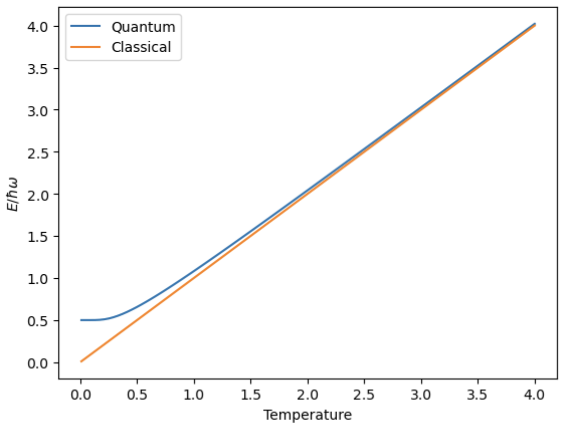
We can see this in the average energy. In the limit of large temperature, the result approaches the equipartition result, in which U = (f/2) k T, with f = 2 in the case of an oscillator. Temperature is plotted in units of the Boltzmann constant.
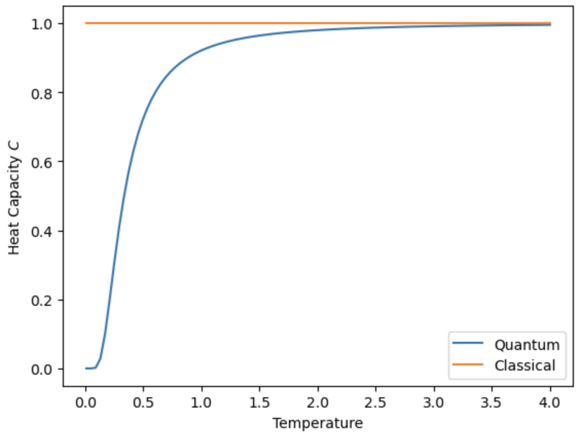
The derivative of the energy is the heat capacity. Below, we see how the
quantum heat capacity behaves vs. the classical heat capacity. Plotted
below is C_{V}/ k.
Recall the plot of the heat capacity as a function of temperature in Chapter 1 of Schroeder (reproduced below)
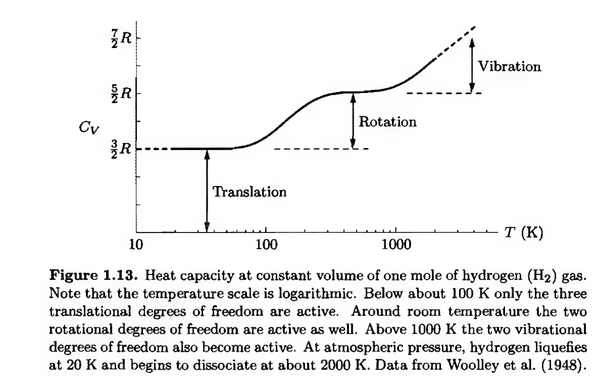
The vibrational contribution can be modeled by a quantum harmonic oscillator. This will enter the partition function multiplicatively:
Z_{tot} = Z_{trans} Z_{rot} Z_{vib}
i.e. the partition function is a product of translations, rotational, and vibrational contributions. The last term Z_{vib} is the quantum partition function defined above. The free energy of each mode is additive:
F_{tot} = F_{trans} + F_{rot} + F_{vib}
And since the heat capacity comes from derivatives of the free energy, it will satisfy:
C_{V} = C_{V}^{trans} + C_{V}^{rot} + C_{V}^{vib}
The blue curve in the figure above shows what C_{V}^{vib} will look like. For small temperatures, there is no contribution - these modes are said to be “frozen out”. For higher temperatures, their contribution approaches R, which accounts for the step in the curve in Fig. 1.13.