You roll two fair dice. How many possible outcomes are there? What are the possible totals? What is the most likely roll?
Generalization of the Quiz: given two n sided die, what is the probability of observing the total T?
The total number of configurations is n^{2}, and the multiplicity for small T is similar to before:
Now listing: T, (n_{1}, n_{2}), and \Omega(T): T = 2; (1, 1); \Omega = 1 T = 3; (1, 2), (2, 1); \Omega = 2
up to
T = n+1; (1, n), (2, n-1), ..., (n, 1), \Omega = n
So for T = 2, ..., n+1, the probability is P(T) = (T - 1)/n^{2}. For T > n+1, we have a reflection symmetry about T = n+1, which can be written
P(T) = P(2n - T + 2) Check a few examples: P(1) = P(2n), P(n) = P(n+2), and also verify that the argument on both sides is the same for T = n+1. Therefore, for T > n+1, we get
P(T) = \frac{2 n - T + 1}{n^{2}}, \quad {\rm for} \quad T > n+1
We can summarize these using absolute value, which can take a straight line and create a tent.
P(T) = \frac{1}{n^{2}} + \frac{n - 1 - | T-1- n|}{n^{2}}
To get this, I used the fact that the tent function from x = 0 to x = 2a, which has a maximum at x =a and goes to zero at x = 0 and x = 2a can be written f(x) = a - |x - a|
Now, define the variable t = T - 2, then define the function
f(t) = P(t + 2) - \frac{1}{n^{2}} we get f(t) = t/n^{2} for t\le n-1, and f(t) = (2 n - 2 - t)/n^{2} for n\le t \le 2n - 2. And f(0) = f(2n-2) = 0. Therefore f(t) is the tent function with a = (n-1).
In the previous few lectures, we discussed the first law of thermodynamics, the ideal gas law, the equipartition theorem, and heat capacity. So this lecture will be a little bit of a right-turn. This can be motivated in the following way: so far we discussed macroscopic phenomena. But macroscopic properties like temperature and pressure can arise from a huge number of microscopic configurations. In other words, particles can wander over a huge space in the position-momentum (x, p) space, but still only have a single P, V, T, since the latter set are averaged macroscopic quantities. Statistical mechanics, in large part, is about accurately counting how many configurations give rise to the same thermodynamic state variables. So, we have to get good at counting. Hence, the heavy emphasis in the next few lectures on combinatorics.
Let me start with the motivation for why we need to get good at counting. It comes down to the fundamental assumption of statistical mechanics:
“In an isolated system in thermal equilibrium, all accessible microstates are equally probable.”
We will use this assumption to actually derive the ideal gas law. But that comes later, for now, we are going to dig into the meaning of these terms.
The simplest starting point is a collection of non-interacting two-level systems.
There are N dipoles, each with possible magnetization s = \pm 1. This is similar to a coin, which can be either heads (+1) or tails (-1). The total magnetization is M= \sum_{i = 1}^{N} s_{i} where s_{i} is the magnetization of the i^{th} dipole.
The microstate is the configuration of spins, (s_{1}, s_{2}, ..., s_{N}). The macrostate is the total magnetization. Let’s take N = 2. There are a total of four microstates, with magnetization (-2, 0, +2). However, they have different degeneracy.
Solution: A fun way to solve the problem is using a generating function. Not the ONLY way. The number of configurations can be gotten in the following way: G(x) = (x + x^{-1})^{N} where x counts the number of dipoles with s = 1, and x^{-1} counts the number of dipoles with s = -1. Basically, we have x^{s} inside the parentheses, for both values of s. Expanding G(x) for N = 3:
G(x, y) = x^{3} + 3 x^{2} x^{-1} + 3 x x^{-2} + x^{-3} = x^{3} + 3 x + 3 x^{-1} + x^{-3}
The exponent of each term tells us the total magnetization, and the coefficient tells us how many configurations there are. So,
M = 3, \quad \Omega = 1 M = 1, \quad \Omega = 3 M = -1, \quad \Omega = 3 M = -3, \quad \Omega = 1
This is just 3/8, which is the same probability as observing the opposite magnetization M = -1.
Solution: I’m going to use the generating function again. It tells us
G(x) = ( x + x^{-1})^{N} = \sum_{q = 0}^{N} \left( { N \atop q}\right) x^{N-2q}
For M = N - 2 q, the multiplicity is \Omega = \left( { N \atop q}\right) = \left( { N \atop (N - M)/2}\right)
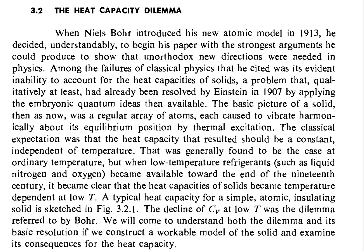
Basic motivation: why it’s called an Einstein Solid. This excerpt is good:
From Goodstein’s book States of Matter:
You know that classical physics predicts a heat capacity which is independent of temperature. And that for ideal gas, heat capacity in experiments shows step-like behavior, depending on temperature. This is just another piece of evidence that classical physics is not sufficient to understand all of the experimental observations in thermodynamics and statistical physics. The Einstein solid is an important first step toward resolving one of these puzzles (vanishing of heat capacity as T \to 0)
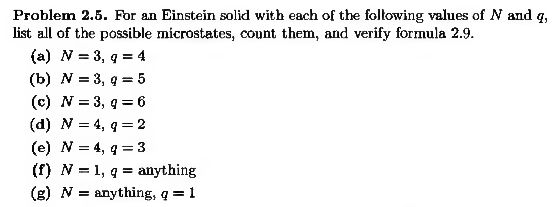
An Einstein solid is a collection of N oscillators, each with a spectrum
E_{i} = \hbar \omega n_{i}, \quad n_{i} = 0, 1, ....,
The total energy of this collection of oscillators is just the sum of individual energies:
E = \hbar \omega \sum_{i = 1}^{N} n_{i} \equiv \hbar \omega q
we say (as in the book) that the ensemble has q total energy units. We start with some examples:
If N = 2, we can enumerate the first few possibilities:
q = 0, \quad \{(0,0)\},\quad \Omega = 1 q = 1, \quad \{ (0,1), (1, 0)\}, \quad \Omega = 2 q = 2, \quad \{ (2, 0), (1, 1), (0, 2)\} , \quad \Omega = 3
…and so forth.
The general formula turns out to be \Omega(N, q) = \left( { N - 1 + q \atop q}\right)
This can be seen from the stars and bars theorems, which were also discussed in Schroeder.
 Solution:
Solution:
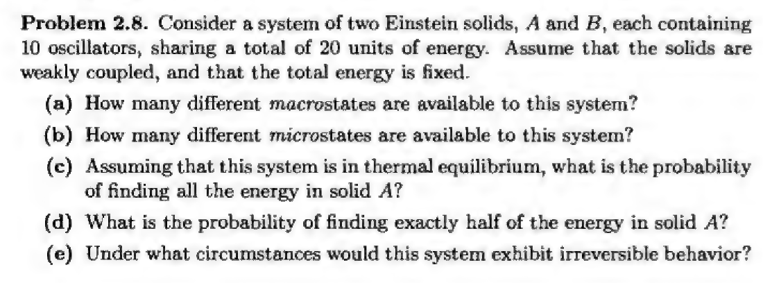
q_{tot} = q_{A} + q_{B} = 20
There are 21 possible values of (q_{A}, q_{B}), e.g. (0, 20), (1, 19), …., (20, 0).