We are interested in what drive a system to reach equilibrium. In the
last class, we considered a spin chain, organized initially in a very
out of equilibrium configuration. Then we turned on interactions, which
were pretty weak, and it started to mix the system, do what is called
thermalize the system. The predictive theory of how this thermalization
occurs is that under a constraint of total energy (or magnetization,
which is equivalent in that example), the system will explore all
accessible microstates with equal probability. Therefore, the macrostate
that wins will just be the most frequent, or that one with the highest
probability mass.
In the process, I almost defined the entropy. I will define the
entropy right now
S(U, N, V) = k_{B} \ln \Omega(U, N, V)
What this says: the entropy, which is a function of the energy,
number of particles, and volume, is equal to k_{B} which is a numerical physical factor,
times the log of the multiplicity of a system at those fixed values. So
when we are talking about maximizing multiplicity, we are also talking
about maximizing entropy. This is why it’s a useful quantity to define.
What is not obvious from this definition is that the entropy will have a
connection to heat flow. That comes later. For now, we are just thinking
about macrostates and microstates, and how to infer the most probable
macrostate - we get this by maximizing entropy.
Let’s extend this now to the ideal gas.
Ideal Gas and Entropy
Quick derivation of multiplicity of ideal gas:
Phase space for each particle is
({\bf x}, {\bf p})
An ideal gas is a collection of free particles. This means the
internal energy per particle is
U = || {\bf p}||^{2}/2m
We also constrain the volume, so that e.g. {\bf x} can only be within a volume V of space. In 1D, we can visualize exactly
what the allowed phase space looks like:
Exercise:
Draw phase space, and show the regions that are allowed by a single
particle.
The allowed configurations consistent with energy and volume
constraints are the blue lines. How many configurations are there? How
many points are there on a real number line? Infinity. In fact, it’s
uncountably infinite.
The solution which the original statistical mechanics proposed is to
quantize the phase space, by saying that phase space is tiled by boxes
of dimension \Delta x \Delta p = h.
Then all the points inside this box count as one configuration. Quantum
mechanics makes this precise, as we will see later in the semester.
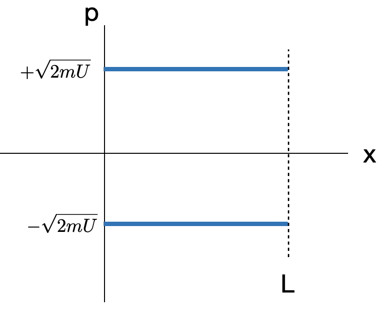 On the interval above, there will be approximately 2L/h in total. In general, the approach is to
compute the area in (x, p), and divide by h. In 3D, phase space is 6 dimensional, and
you would again compute the volume in x
and the volume in p, and divide by
h^{3}. This leads to the formula in the
book
On the interval above, there will be approximately 2L/h in total. In general, the approach is to
compute the area in (x, p), and divide by h. In 3D, phase space is 6 dimensional, and
you would again compute the volume in x
and the volume in p, and divide by
h^{3}. This leads to the formula in the
book
\Omega_{1} = \frac{V V_{p}}{h^{3}}
For the 1D gas, we have V = L. What is
the right way to compute V_{p}?
2m U = \sum_{i = 1}^{N} p_{i}^{2}
The volume in phase space at fixed radius r^{2} = \sum_{i} p_{i}^{2} scales like V_{p} =r^{N - 1} d\Omega , so replacing r^{2} \sim U gives V_{p} \sim U^{(N-1)/2}
Putting it together,
\Omega_{N} \sim f(N) U^{(N-1)/2} V^{N}
which is the main result.
Thermal Equilibrium and
Multiplicity
A very important property of weakly interacting systems is that
entropy is additive. Consider two subsystems A and B. The
combined system AB has a multiplicity
given by
\Omega_{AB} = \Omega_{A}
\Omega_{B}
Which means S_{AB} = S_{A} +
S_{B}
Now we make the crucial assumption
Exercises
If A starts with internal energy
U_{A}, and B starts with internal energy U_{B}, and both have the same volume,
what is the total energy? U = U_{A} +
U_{B}
What is the internal energy of subsystem A after the two systems have interacted for a
long time?
We find this by looking at the multiplicity. The multiplicity is
\Omega = \Omega_{A} \Omega_{B} = f(N)^{2} V^{2N} U_{A}^{fN/2}
U_{B}^{fN/2}
The two systems cannot exchange particles, and their volume is
fixed. They can really only exchange entropy. Since the total
energy is fixed, we can write the multiplicity as a continuous
function
\Omega = {\rm stuff} \times \left( (U - U_{A}) U_{A}\right)^{fN/2}
To see how this behaves, I will write x = U_{A}/U. Then the multiplicity can be
written
\Omega = stuff\times (x (1 - x))^{fN/2}
Since V and N are fixed, x is really the only variable left in the
problem. And this formula shows that \Omega(x) takes its maximum value at x = 1/2, for which U_{A} = U_{B} = U/2.
Let’s revisit the problem above, but ask about change in entropy.
S_{A} = S(N,V)+ \frac{N f}{2} \ln U_{A}, \quad S_{B} = S(N, V) + \frac{N
f}{2} \ln U_{B}
Afterward,
\Omega_{tot} = \omega(N, V)^{2} U^{f (2N)/2}
which means
S_{f} = 2 S(N, V) + \frac{f N}{2} \log (U^{2})
The change in entropy is
S_{f} - S_{i} = \frac{f N}{2} \left[ \ln U^{2} - \ln U_{A} - \ln
U_{B}\right]
Using x = U_{A}/U, this becomes
\ln \frac{U^{2}}{ ( U_{A}(U - U_{A}))} = \ln\frac{1}{ x (1 - x) } = -
\ln x (1 - x) > 0
Which is all we need to show.
Heat and Entropy
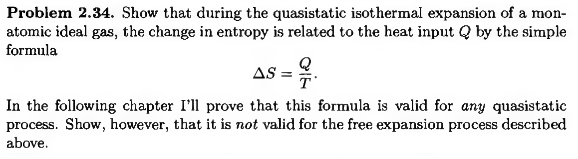 Solution: I like this problem because it requires combining the
first law with the ideal gas law, and even a bit of the equipartition
theorem.
Solution: I like this problem because it requires combining the
first law with the ideal gas law, and even a bit of the equipartition
theorem.
Relevant formulas:
The volume dependence of the entropy is S(N, V, U) = N \ln V + g(N, U)
- Let’s compute work: for quasistatic isothermal expansion, we have
W_{by\, gas} = \int P dV = N k T \log V_{f}/V_{i}
The internal energy doesn’t change, so
Q = W_{by \, gas} = N k T \log V_{f}/V_{i}
Next, independently, we can calculate the change in entropy.
Importantly, entropy is a state function, and therefore
the change only depends on the end-points if the process is
quasi-static. Knowing the relevant dependence on the volume, we get
\Delta S = N k \ln (V_{f}/V_{i})
Comparing to the heat, we get
\Delta S = \frac{Q}{T}
- Does gravity cause entropy to decrease?
Under the universal law of gravitation, a collection of massive
classical particles will, generically, collapse to a point. This would
seem to violate the second law of thermodynamics, which states that the
entropy of a closed system must never decrease. If massive particles
inevitably collapse to a point, their available microstates apparently
shrinks, and thus the entropy shrinks as well. The resolution to this
puzzle is discussed quite nicely in the following pedagogical paper:
https://arxiv.org/html/2604.24780v2
Briefly, the escape hatch for this paradox is that matter that is
collapsing under gravity to a point is also accelerating, and
accelerating particles emit radiation. The entropy lost to local massive
particle ordering is dumped into the radiation that is emitted into the
universe.
- Does black hole entropy count microstates? TBD…