In Lecture 6 , you looked at the multiplicity of a two-state paramagnet. The result for the multiplicity at fixed magnetization
\Omega(N,U) = \left( { N \atop \frac{1}{2}(N + U/E_{0})}\right) Where E_{0} = m_{0}B was the energy of a single magnetic moment m_{0} in a magnetic field B.
The magnetization is M = \sum_{i = 1}^{N} s_{i} and the energy is U = - E_{0} M.
Exercise: 1) Find the entropy for large N and zero energy U = 0 . Use Stirling’s approx to leading order. Recall that the Stirling approximation is best understood as an asymptotic expansion of the log of the factorial:
\ln N! = N \ln N - N + \frac{1}{2} \ln N + O(1) Each successive term is smaller.
Solution: At M = 0, \Omega = \left( { N \atop N/2}\right) = \frac{N!}{\left(( N/2)! \right)^{2}}, and so
S/k = \ln N! - 2 \ln (N/2)! and for large N, Stirling’s approximation gives
S/k = N \ln N - N + \frac{1}{2} \ln N - 2 \left( \frac{N}{2} \ln \frac{N}{2} - \frac{N}{2} + \frac{1}{2} \ln N/2\right) = N \ln 2 - \frac{1}{2} \ln N + O(1) The dominant term is linear in N, and proportional to \ln 2.
Solution:
There are a total of 2^{N} configs, so that \Omega = 2^{N} and S = N k \ln 2.
This result suggests that approximately all configurations are accessible at U = 0 at finite magnetic field. The dominant linear in N contribution is the same for both. However, the entropy at U = 0 and B>0 computed in (1), is strictly smaller than the B = 0, U = 0 entropy computed in (2). This makes sense, because (2) is the largest possible value the entropy of this system can take. Now writing entropy as a function of U and B, S(U, B), I get
S( 0, B)= S(U,0) - \frac{1}{2} \ln N
Note also that S(U) is maximal at U = 0 for this system. This means this corresponds to infinite temperature. Another interpretation then is that at infinite temperature, the magnetization will vanish even for finite magnetic field. This is essentially because in this limit, each spin becomes an independently fluctuating variable which has on average a zero dipole moment.
Treating the magnetic field as a thermodynamic variable is a bit jumping the gun - we’ll get to that much later in the semester. For now, we focus on the thermodynamic variables that are more familiar: energy, number, and volume.
As in Exercise 2.42, the entropy of a black hole is a quadratic function of energy: S\sim U^2. Its temperature therefore scales as
T\sim\frac{1}{U}.
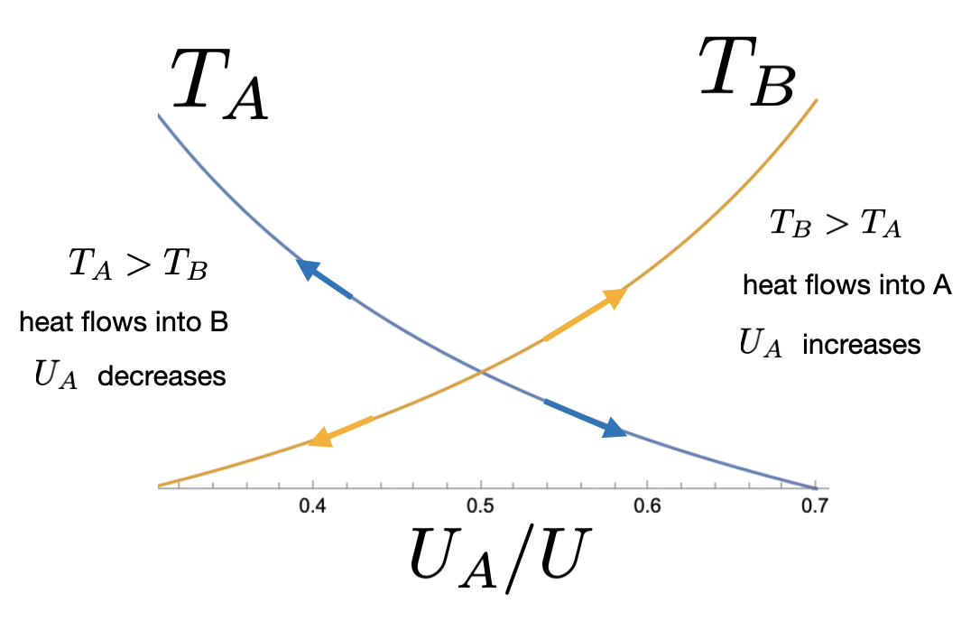
For two such systems A and B with total energy U=U_A+U_B, does an equilibrium exist? Will systems starting at different energies reach it?
The temperature curves as functions of U_A/U intersect at equal energies. To the left of the intersection, T_A>T_B, heat flows into B, and U_A decreases. To the right, T_B>T_A, heat flows into A, and U_A increases. The intersection exists, but any small energy imbalance drives the systems farther from it: the equilibrium is unstable.
The figure below shows the temperature for the two systems as a function of the energy U_{A} of the subsystem.
Consider two spin systems, one prepared at -T, one at +T. What will their final temperature be?
For an ideal gas,
S\sim\frac{Nfk}{2}\ln U, \qquad \frac{1}{T}=\frac{Nfk}{2U}, \qquad U=\frac{Nf}{2}kT.
The last result agrees with equipartition. For two identical subsystems with U=U_A+U_B,
T_A=\frac{2U_A}{Nfk}, \qquad T_B=\frac{2U_B}{Nfk}=\frac{2(U-U_A)}{Nfk}.
As functions of U_A/U, these are straight lines that intersect at U_A/U=1/2. On the left, T_B>T_A, heat flows into A, and U_A increases. On the right, T_A>T_B, heat flows out of A, and U_A decreases. Both directions lead toward the intersection, so the equilibrium is stable.
The figure below shows the temperature for the two systems as a
function of the energy U_{A} of the
subsystem. 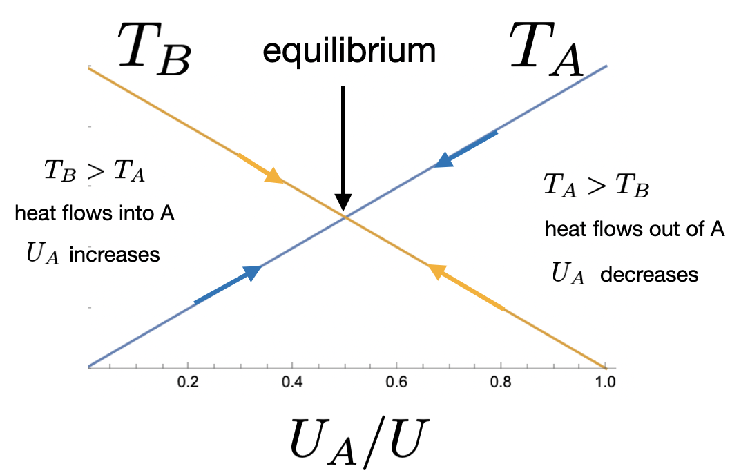
Let us look at what happens when two paramagnetic systems come into thermal contact. Assume both have N dipoles, but they are initially isolated and at different energies U_{1}^{init} and U_{2}^{init}. After contact, the total energy will be U = U_{1}^{init} + U_{2}^{init}. Thermal equilibrium is reached when:
\frac{\partial S_{1}}{\partial U_{1}} = \frac{\partial S_{2}}{\partial U_{2}} Since the total number of dipoles is the same for both, the entropy for both is given by S_{1} = S(U_{1}, N), and S_{2} = S(U_{2}, N). In other words, they are the same function. The derivatives become equal when U_{1} = U_{2}. That implies each system will reach the energy U_{1} = U_{2} = \frac{1}{2} U = \frac{1}{2} \left( U_{1}^{init} + U_{2}^{init}\right). In words, they equilibrate to their average energy. Let us look more closely at what this would like in some scenarios:
Imagine U_{1}^{init} < U_{2}^{init}
< 0. Then T_{1}^{init} <
T_{2}^{init}, and conventional thinking tells us that system 2
will lose heat to system 1. This will cause U_{2} to decrease, while U_{1} increases. 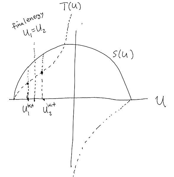
U_{1}^{init} < 0 <
U_{2}^{init}. In this case, T_{1}^{init} > 0, and T_{2}^{init} < 0. We can no longer apply
the conventional thinking. The final equilibrium energy of each
subsystem is still the average energy, so we have again that system 2
will lose heat to system 1, raising the temperature of system 1. 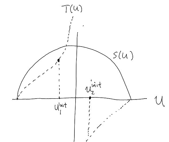
U_{1}^{init} < U_{2}^{init} = 0. In this case, System 2 is at infinite temperature. What will happen? The very same thing: system 2 loses heat to system 1, bringing its temperature down to a finite value.
A final example: 0 < U_{1}^{init}
< U_{2}^{init}. Now, we have again that T_{2}^{init} > T_{1}^{init}, and in fact
the conventional thinking applies again! As in every case above, system
2 loses heat (and thus energy) to system 1. 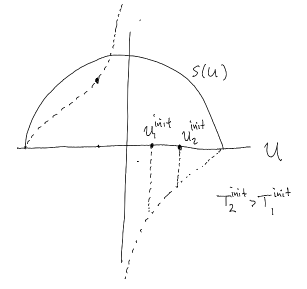
What’s the take-away? With spin systems, in order to understand heat flow, the reliable approach is to think about equilibrium using entropy. This is because of the highly unintuitive fact that negative temperature systems will always give up heat to positive temperature systems.
Entropy is a thermodynamic state function, which depends on these three thermodynamic variables: S(U, N, V) Therefore, we can relate changes in entropy to changes in any of these three thermodynamic variables by using the chain rule along with partial derivatives, making sure to fix the appropriate variables:
dS = \left( \frac{\partial S}{\partial U}\right)_{N,V} d U + \left( \frac{\partial S}{\partial V}\right)_{U, N} dV + \left( \frac{\partial S}{\partial N}\right)_{U,V} dN \tag{1}
We already know that the temperature is defined via:
\frac{1}{T} = \left( \frac{\partial S}{\partial U}\right)_{N,V}
Next, we can identify which thermodynamic variables the other partial derivatives are calculating. If we take for now dN = 0 (which corresponds to a process that involves a fixed quantity of stuff), we get from (1):
dS = \frac{1}{T} dU + \left( \frac{\partial S}{\partial V}\right)_{U, N} dV
We will match this to the first law of thermodynamics to interpret the partial derivative and the differential of the entropy. For the work done by a differential change in volume, we get dW = - P dV (check the sign: if the volume change is positive, the gas is doing work, and losing energy from doing such work, so this sign is correct). Therefore, the first law gives us
dU = Q + W = Q - P dV = T dS - T \left( \frac{\partial S}{\partial V}\right)_{U,N} dV Now matching terms, we can identify first what the differential of heat must look like
Q = T dS
and that the pressure can be defined in terms of entropy!
\boxed{P = T \left( \frac{\partial S}{\partial V}\right)_{U,N}}
This is a shortcut to the thermodynamic identity, but it’s not generally true. In particular, identifying Q = T dS is only correct for quasistatic processes. In general, the thermodynamic identity and the first law of thermodynamics are independent, and both generally true. Combined, they imply that in general
dS \ge \frac{Q}{T}
Intensive: state variable that is independent of system size. These are the variables that determine equilibrium between two bodies: - Temperature T - two systems share a temperature when they are in thermal equilibrium, regardless of their size and composition - Pressure P - two systems are in mechanical equilibrium (forces are balanced) when they have same pressure. - Chemical Potential \mu - determines diffusive equilibrium
Extensive: state variable that grows with system size, keeping intensive variables fixed. Examples include: - Internal Energy U - Entropy S - Volume V - Number of Particles N