 At constant entropy, the thermodynamic identity gives
We have been thinking a lot about thermodynamic variables. These are the variables that completely specify the macroscopic state of a system. We found a number of them. Let’s list them out:
When a system, like a gas, is in thermal equilibrium, it has a well defined state, and all of the state variables are well-defined.
Furthermore, they are not all independent. As we have seen, there will be an equation of state that relates them, e.g. the ideal gas law:
PV = N k T It is particularly useful to treat entropy as a state-function, even though it could just as well be a state variable. More specifically, we found in thinking about the multiplicity of a dilute gas that the entropy is determined by the total number of particles N, the total volume in space V, and the total internal energy U. Therefore, entropy is a function of these three state variables:
S(U, V, N)
The thermodynamic identity comes from this fact: if you have a state function, and want to think about differential changes in the state function, you can relate this to changes in each of its variables:
dF(x_{1}, x_{2}, x_{3}) = \partial_{x_{1}} F d x_{1} + ... = \left(\nabla F\right) \cdot d{\bf x}
This is familiar in 1D:
d F(x) = \left(\partial_{x} F\right) dx
This also has another consequence: To compute the difference over a trajectory, we just integrate along that trajectory:
\int_{1}^{2} dF = F(2) - F(1) Because dF is an exact differential, the integral is just equal to the difference between F evaluated at the endpoints.
This is a generalization of the familiar rule in 1D:
\int_{x_{1}}^{x_{2}} dF(x) = \int_{x_{1}}^{x_{2}} \partial_{x}F dx = F(x_{2}) - F(x_{1})
In multivariable calculus, it’s called the Gradient Theorem.
But what type of trajectories does this make sense for? It is for trajectories in which there are well-defined thermodynamic variables throughout. This will be true for quasi-static trajectories, i.e. ones taken very very slowly, so that at each moment the system is in equilibrium.
As I mentioned in Lecture 4, the first law involves differentials that are not exact differentials - these are heat and work.
dU = \delta Q + \delta W This means that when integrated between two fixed endpoints, the final value of the path integral will be path dependent:
(N.B. The bar over the d is just to remind you that they are inexact differentials. A more common notation is a d with a slash through it. Again, only to remind you that these are not exact differentials )
This is because Q and W are not state variables, and do not come from the derivative of a potential function. They depend on the path you take, and not just on the endpoints. But there can still be a differential amount of them.
Work done by an electric field. The force is the coulomb force {\bf F} = q {\bf E}, and since it is a conservative force {\bf F} = - q \nabla \Phi, where \Phi is the electrostatic potential. The work done by the Coulomb force is
W = \int_{1}^{2} {\bf F} \cdot d {\bf r} = - q \int_{1}^{2} d\Phi = - q \left( \Phi(2) - \Phi(1)\right)
This is exactly because {\bf F} is conservative. So \delta W = - q d\Phi is an exact differential in this case, because it is produced by a conservative force.
What about work done in thermodynamics? For a quasi-static process, we have that the substance does the following work:
W = - \int P(V) dV
The problem here is that there is no single “potential” whose difference defines the work done. Of course, we can construct the anti-derivative of P(V). But there will be many different possible anti-derivatives, each depending on the path taken in the state space. So for this reason, \delta W is an inexact differential, and its integral is path dependent.
Writing entropy as a state function as above, taking infinitesimal displacements of all of its arguments,
dS = S(U + dU, V + dV, N + dN) - S(U, V, N)
And expanding to linear order in all the differentials, gives dS = \left( \frac{\partial S}{\partial U}\right)_{N,V} d U + \left( \frac{\partial S}{\partial V}\right)_{U, N} dV + \left( \frac{\partial S}{\partial N}\right)_{U,V} dN, \quad (1)
If our system undergoes some process as a trajectory in the (U, V, N) space, then we would use this relation to determine the change in entropy along this process. Let us denote \Delta S as the net (non-infinitesimal) change in entropy. Then we get this by integrating dS
\Delta S = \int_{1}^{2} dS With the control integral taken over some path in the 3 dimensional (U, V, N)-space. Since dS is an exact differential, the integral will evaluate to be a difference between endpoints:
\Delta S = S(2) - S(1)
In this sense, perhaps trivially, since entropy is a state function, and therefore dS is an exact differential, changes in entropy are path independent. For these reasons, we may refer to entropy as a thermodynamic potential, akin to the electrostatic potential in the example earlier. We will dive much deeper into this concept in Chapter 5.
The differential relation above is often written in a way to feature the energy. This is motivated by its connection to the first law of thermodynamics. In other words, we have for the first law:
dU = \delta Q +\delta W
For a system that allows variable number of particles, we must add to the mechanical work - P dV a chemical work \mu dN, so that the first law reads
dU = \delta Q - P dV + \mu dN
Comparing to (1), we can identify the following partial-derivative relations for pressure:
\boxed{P = T \left( \frac{\partial S}{\partial V}\right)_{U,N}}
and chemical potential:
\boxed{\mu = -T \left( \frac{\partial S}{\partial N}\right)_{U,V}}
What remains is the connection between heat and entropy. By using the definition of temperature
\boxed{\frac{1}{T} = \left( \frac{\partial S}{\partial U}\right)_{V,N}}
We may identify, again using (1) and the first law:
\delta Q = T dS
We could have proceeded slightly differently. Let us assume that we did not know ahead of time how to identify the partial derivative of S wrt U. If we didn’t know ahead of time, we might just define it
\beta = \left( \frac{\partial S}{\partial U}\right)_{V, N}
Eq. (1) and the first law imply then that
\delta Q = \frac{1}{\beta} dS
Now let’s consider a simple setting in order to figure out what thermodynamic variable \beta is. Let us consider a simple isothermal expansion. In this case, we can use the Sackur-Tetrode formula for the entropy of a gas to get the change in entropy as
\Delta S = N \log (V_{f}/V_{i})
Similarly, the work done by the gas, and thus the heat flow into the gas, is given by
W^{by\, \, gas} = N k T \ln \left( V_{f}/V_{i}\right) = Q
Compare these results gives
Q = \frac{\Delta S}{T} \Rightarrow \beta = 1/T
This is an example of using results from thermodynamics to identify thermodynamic variables in statistical mechanics.
We solved this problem also in Lecture 7.
At constant entropy, the thermodynamic identity gives
dU = T dS - P dV+ \mu dN
Fixing entropy means dS = 0. That is, we are considering displacements along a constant entropy hypersurface. Along this surface, the thermodynamic identity implies
dU = - P dV + \mu dN This suggests that the natural variables for the energy are V, N, i.e. U = U(V, N), and that
dU = \left( \frac{\partial U}{\partial V}\right)_{N, S} dV + \left( \frac{\partial U}{\partial N}\right)_{S, V} dN
Comparing with the thermodynamic identity gives
P = - \left( \frac{\partial U}{\partial V}\right)_{N, S}
Enthalpy was introduced in the previous chapter. It is defined H = U + PV It is a convenient way to define heat capacity at constant pressure:
C_{P} = \left( \frac{\partial H}{\partial T}\right)_{P} This is all you need for the exercises below.
Exercise: Find an expression for dH in terms of dS and dP using the thermodynamic identity:
Solution:
dH = dU + d ( PV) = dU + P dV + V dP Now substituting dU = T dS - P dV, we get
dH = TdS + V dP
This will be useful to solve the next problem:
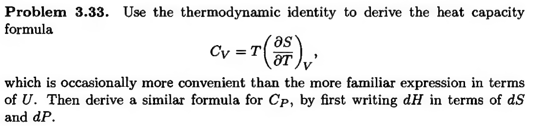
Solution: At constant volume and number, the thermodynamic identity implies
dU = T dS, \quad dV = dN = 0 At constant volume, the heat capacity is
C_{V} = \left( \frac{\partial U}{\partial T}\right)_{V} \quad (1)
Let us assume the energy is a function of T, V, N, U = U(T, V, N), and similarly the entropy S = S(T, V, N). When we consider differentials of U and S, we will get, e.g.
dU = \left( \frac{\partial U}{\partial T}\right)_{V,N} dT + \left( \frac{\partial U}{\partial V}\right)_{T,N} dV + \left( \frac{\partial U}{\partial N}\right)_{T,V} dN and similarly dS = \left( \frac{\partial S}{\partial T}\right)_{V,N} dT + \left( \frac{\partial S}{\partial V}\right)_{T,N} dV + \left( \frac{\partial S}{\partial N}\right)_{T,V} dN
Next, since dU = TdS for dV = dN = 0, we can compare the coefficients of dT to get \left( \frac{\partial U}{\partial T}\right)_{V,N} = T \left( \frac{\partial S}{\partial T}\right)_{V,N}
A much simpler heuristic to get the same result is that we can start with dU = TdS, and just “divide by dT” on both sides.
Next, for a constant pressure process, we get the formula for the heat capacity
C_{P} = \left( \frac{\partial U}{\partial T}\right)_{P,N} + P\left( \frac{\partial V}{\partial T}\right)_{P,N} = \left( \frac{\partial \left( U + P V\right)}{\partial T}\right)_{P,N} = \left( \frac{\partial H}{\partial T}\right)_{P,N}
where H is the enthalpy. But at constant P, the thermodynamic identity for enthalphy implies
dH = TdS + V dP = TdS , \quad {\rm when}\, \, dP = 0
So
C_{P} = \left( \frac{\partial H}{\partial T}\right)_{P,N} = T \left( \frac{\partial S}{\partial T}\right)_{P,N} Which is a nearly identical formula.

Approach 1: Let’s approach this problem starting with only the very basics:
Let us do it the hard way:
dS = \frac{1}{T} \left( dU + P dV\right) So that integrating along this path gives
\Delta S = \int \frac{dU}{T} + \int \frac{P dV}{T} Next, using PV = N k T , and dU = \frac{f}{2} N k dT gives
\Delta S = \frac{f}{2} \int \frac{N k dT}{T} + \int \frac{N k dV}{ V}
Evaluating gives
\Delta S = \frac{f N k }{2} \ln T_{f}/T_{i} + N k \ln V_{f}/V_{i} Next, use the ideal gas law gives:
\frac{V_{i}}{T_{i}} = \frac{V_{f}}{T_{f}}
which implies
\frac{V_{f}}{V_{i}} = \frac{T_{f}}{T_{i}} And finally, we can write the change in entropy in terms of the change in temperature
\Delta S = \frac{(f + 2) }{2} N k \ln T_{f}/T_{i} Now I use the fact that the isobaric heat capacity C_{P} = \frac{(f+2)}{2} N k. Also, if the volume doubles, then so does the temperature, which gives the final result: \Delta S = C_{P} \ln 2
Approach 2: Another approach is to use the definition of heat capacity:
C_{V} = \left( \frac{\partial Q}{\partial T}\right)_{V} = \left( \frac{\partial U}{\partial T}\right)_{V} = \frac{f }{2} N k (this is Schroeder Eq. 1.46)
And the constant pressure version
C_{P} = \left( \frac{Q}{\Delta T}\right)_{P} = \frac{d U + P dV}{dT} = \frac{T d S}{dT}
Here we used the first law to rewrite Q = dU + P dV for a reversible process, and then the thermodynamic identity to rewrite this as T dS. This then implies
dS = \frac{C_{P}}{T} dT
Integrating this along the path then immediately gives: \Delta S = C_{P} \ln T_{f}/T_{i}, as we got above.